🎯 نواتج التعلم
🎯 Learning Outcomes
بعد دراسة هذا الدرس ستكون قادرًا على أن:
After this lesson you will be able to:
- تكتب الأعداد الكبيرة جدًا والصغيرة جدًا بالترميز العلمي \(a\times10^{n}\) وتجري عليها الضرب والقسمة.Write very large and very small numbers in scientific notation \(a\times10^{n}\) and multiply and divide them.
- تعدّد الكميات الأساسية ووحداتها في النظام الدولي (SI) وتميّزها من الوحدات المشتقة.List the base quantities and units of the SI system and tell them from derived units.
- تستخدم بادئات الوحدات (كيلو، ملي، ميكرو …) وتحوّل بين الوحدات بمعامل التحويل.Use unit prefixes (kilo, milli, micro …) and convert between units with a conversion factor.
- تتحقق من صحة علاقة فيزيائية بالتحليل البعدي.Check a physical relation with dimensional analysis.
- تعدّ الأرقام المعنوية وتطبّق قواعد الضرب والقسمة والجمع والطرح عليها.Count significant figures and apply the rules for multiplication, division, addition and subtraction.
- تميّز بين الدقة والضبط، وتكتب القراءة مع هامش الخطأ.Tell accuracy from precision and write a reading with its margin of error.
- ترسم العلاقات بين المتغيرات وتحسب الميل وتميّز العلاقة الطردية والخطية والعكسية.Plot relations between variables, compute the slope and tell direct, linear and inverse relations.
📐 الترميز العلمي
📐 Scientific Notation
لماذا نستخدم الترميز العلمي؟ لأن الفيزياء تتعامل مع أعداد كبيرة جدًا (كتلة الأرض وحجم المجرات) وصغيرة جدًا (شحنة الإلكترون وحجم الذرة)، وكتابتها بأصفارها الكثيرة مرهقة ويسهل الخطأ فيها؛ فالترميز العلمي يمثّلها بسهولة وبشكل مختصر.
Why do we use scientific notation? Physics deals with huge numbers (the mass of the Earth, the size of galaxies) and tiny ones (the charge of the electron, the size of an atom). Writing them with all their zeros is tiring and error-prone; scientific notation represents them easily and compactly.
🌍 مثال 1: كتلة الأرض
🌍 Example 1: The mass of the Earth
كتلة الأرض تعادل تقريبًا \(5972000000000000000000000\ kg\). نكتبها على الصورة \(5.972\times1000000000000000000000000\)، والعدد \(1000000000000000000000000\) هو الذي يسبّب المشكلة فهو من مضاعفات العشرة؛ إنه \(1\) متبوعًا بـ \(24\) صفرًا، أي حاصل ضرب \(24\) عاملًا كلّ منها \(10\):
The mass of the Earth is about \(5972000000000000000000000\ kg\). We write it as \(5.972\times1000000000000000000000000\); the troublesome number \(1000000000000000000000000\) is a power of ten: a \(1\) followed by \(24\) zeros, i.e. the product of \(24\) factors each equal to \(10\):
🔟 قوى العشرة
🔟 Powers of ten
\[10=10^{1},\quad 10\times10=10^{2},\quad 10\times10\times10\times10=10^{4},\;\dots,\quad \underbrace{10\times10\times\cdots\times10}_{24\ \text{factors}}=10^{24}\]
\[m_{\text{Earth}}=5.972\times10^{24}\ kg\]
⚛️ مثال 2: شحنة الإلكترون
⚛️ Example 2: The charge of the electron
شحنة الإلكترون تعادل \(0.00000000000000000016\ C\). نكتبها \(1.6\div10000000000000000000\) أي \(1.6\times\dfrac{1}{10^{19}}\). وبما أن \(\dfrac{1}{10}=10^{-1}\) و\(\dfrac{1}{100}=10^{-2}\) و\(\dfrac{1}{100000}=10^{-5}\) فإن \(\dfrac{1}{10000000000000000000}=10^{-19}\) ومنه:
The charge of the electron is \(0.00000000000000000016\ C\). We write it as \(1.6\div10000000000000000000\), i.e. \(1.6\times\dfrac{1}{10^{19}}\). Since \(\dfrac{1}{10}=10^{-1}\), \(\dfrac{1}{100}=10^{-2}\) and \(\dfrac{1}{100000}=10^{-5}\), then \(\dfrac{1}{10000000000000000000}=10^{-19}\), hence:
⚛️ شحنة الإلكترون
⚛️ The electron charge
\[q=1.6\times10^{-19}\ C\]
📌 صيغة الترميز العلمي وقاعدة النقل
📌 The form and the shifting rule
\[N=a\times10^{n},\qquad 1\le a\lt 10,\quad n\in\mathbb{Z}\]
الفكرة: نحرّك الفاصلة العشرية حتى تقع بعد أول رقم غير صفري من اليسار، فنحصل على العدد \(a\)، ونعدّ الخانات التي تحرّكناها فتعطينا الأس \(n\).
The idea: move the decimal point until it sits just after the first non-zero digit from the left; this gives the number \(a\), and the count of places we moved is the exponent \(n\).
- الفاصلة تحرّكت نحو اليسار (عدد كبير): الأس موجب. مثال: \(98700000=9.87\times10^{7}\) (٧ خانات).The point moved left (a large number): the exponent is positive. Example: \(98700000=9.87\times10^{7}\) (7 places).
- الفاصلة تحرّكت نحو اليمين (عدد صغير أقل من 1): الأس سالب. مثال: \(0.0000007=7\times10^{-7}\) (٧ خانات).The point moved right (a small number below 1): the exponent is negative. Example: \(0.0000007=7\times10^{-7}\) (7 places).
- إذا كان العدد بين \(1\) و\(10\) فالأس \(0\): \(4.5=4.5\times10^{0}\).If the number is between \(1\) and \(10\) the exponent is \(0\): \(4.5=4.5\times10^{0}\).
جرّب بنفسك في التجربة التالية: اكتب أي عدد (أو اختر مثالًا جاهزًا) وراقب كيف تتحرك الفاصلة ويتكوّن الأس.
Try it yourself in the next experiment: type any number (or choose a ready example) and watch how the decimal point moves and how the exponent forms.
🧪 تجربة 1: أين تذهب الفاصلة؟ (الترميز العلمي)
🧪 Experiment 1: Where does the decimal point go? (Scientific notation)
اكتب عددًا عاديًا (كبيرًا أو صغيرًا) أو اختر مثالًا جاهزًا؛ يلوّن البرنامج أول رقم غير صفري ويضع علامة الفاصلة الجديدة ثم يحسب عدد الخانات التي تحرّكتها الفاصلة والأس \(n\). وفي الأسفل حوّل في الاتجاه المعاكس: من \(a\times10^{n}\) إلى العدد العادي.
Type an ordinary number (large or small) or choose a ready example; the program colours the first non-zero digit, marks the new decimal point and counts how many places it moved to get the exponent \(n\). Below, convert the other way: from \(a\times10^{n}\) back to the ordinary number.
↩️ من الترميز العلمي إلى العدد العادي↩️ From scientific notation to the ordinary number
✖️➗ العمليات على الأعداد بالترميز العلمي
✖️➗ Operations on numbers in scientific notation
💡 قاعدتان تُسهّلان الحساب
💡 Two rules that simplify calculation
\[(a\times10^{m})(b\times10^{n})=(a\,b)\times10^{m+n},\qquad \dfrac{a\times10^{m}}{b\times10^{n}}=\dfrac{a}{b}\times10^{m-n}\]
في الضرب نجمع الأسس، وفي القسمة نطرح الأسس. وإذا خرج الناتج عن الصيغة \(1\le a\lt 10\) أعدنا ضبطه (نقلنا الفاصلة وغيّرنا الأس).
In multiplication we add the exponents, in division we subtract them. If the result leaves the form \(1\le a\lt 10\) we re-normalise it (move the point and change the exponent).
- \((3\times10^{4})(2\times10^{3})=6\times10^{7}\)\((3\times10^{4})(2\times10^{3})=6\times10^{7}\)
- \((5\times10^{3})(4\times10^{2})=20\times10^{5}=2\times10^{6}\) (أعدنا الضبط)\((5\times10^{3})(4\times10^{2})=20\times10^{5}=2\times10^{6}\) (re-normalised)
- \(\dfrac{6\times10^{8}}{3\times10^{-2}}=2\times10^{8-(-2)}=2\times10^{10}\)\(\dfrac{6\times10^{8}}{3\times10^{-2}}=2\times10^{8-(-2)}=2\times10^{10}\)
اكتب الأعداد التالية بالترميز العلمي. الضغط داخل عمق البحر \(98700000\ Pa\) يساوي:
Write the following in scientific notation. The pressure deep in the sea \(98700000\ Pa\) equals:
شحنة كرة من الحديد تساوي \(0.0000007\ C\). بالترميز العلمي تكتب:
The charge of an iron ball is \(0.0000007\ C\). In scientific notation it is written:
سرعة الضوء في الفراغ \(300000000\ m/s\). بالترميز العلمي:
The speed of light in vacuum is \(300000000\ m/s\). In scientific notation:
نصف قطر الذرة يعادل تقريبًا \(0.0000000025\ m\). بالترميز العلمي:
The radius of an atom is about \(0.0000000025\ m\). In scientific notation:
🧪 الوحدات الأساسية في النظام الدولي
🧪 Base Units in the International System (SI)
اتفق العلماء في النظام الدولي للوحدات (SI) على سبع كميات أساسية لكل منها وحدة أساسية، ومنها اشتُقّت وحدات جميع الكميات الفيزيائية الأخرى. الجدول التالي يبيّنها:
Scientists agreed in the International System of Units (SI) on seven base quantities, each with a base unit; from them the units of all other physical quantities are derived. The table shows them:
| الكمية الأساسيةBase quantity | الوحدة الأساسيةBase unit | رمز الوحدةSymbol |
|---|---|---|
| الطولLength | المترmetre | m |
| الكتلةMass | الكيلوجرامkilogram | kg |
| الزمنTime | الثانيةsecond | s |
| درجة الحرارةTemperature | كلفنkelvin | K |
| التيار الكهربائيElectric current | أمبيرampere | A |
| شدة الإضاءةLuminous intensity | شمعة (كانديلا)candela | cd |
| كمية المادةAmount of substance | مولmole | mol |
🧠 توضيح: الوحدات الأساسية والمشتقة
🧠 Clarification: base and derived units
الوحدات المشتقة تُبنى بضرب وقسمة الوحدات الأساسية، ولها أحيانًا أسماء خاصة:
Derived units are built by multiplying and dividing base units, and sometimes have special names:
- السرعة: \(m/s\) | العجلة: \(m/s^{2}\) | المساحة: \(m^{2}\) | الكثافة: \(kg/m^{3}\)Speed: \(m/s\) | acceleration: \(m/s^{2}\) | area: \(m^{2}\) | density: \(kg/m^{3}\)
- القوة: النيوتن \(N=kg\cdot m/s^{2}\)Force: the newton \(N=kg\cdot m/s^{2}\)
- الطاقة: الجول \(J=N\cdot m=kg\cdot m^{2}/s^{2}\) | الضغط: الباسكال \(Pa=N/m^{2}=kg/(m\cdot s^{2})\)Energy: the joule \(J=N\cdot m=kg\cdot m^{2}/s^{2}\) | pressure: the pascal \(Pa=N/m^{2}=kg/(m\cdot s^{2})\)
⚠️ الكيلوجرام هو الوحدة الأساسية للكتلة (وليس الجرام)، وهو الوحيد الذي يحمل بادئة في اسمه؛ لذلك \(1\ kg=10^{3}\ g\).
⚠️ The kilogram (not the gram) is the base unit of mass, and it is the only one with a prefix in its name; therefore \(1\ kg=10^{3}\ g\).
🔢 البادئات
🔢 Prefixes
البادئات هي أجزاء ومضاعفات لوحدات القياس، نضعها قبل رمز الوحدة لنختصر كتابة الأعداد الكبيرة والصغيرة؛ فبدل \(0.000000005\ s\) نكتب \(5\ ns\)، وبدل \(6300000\ m\) نكتب \(6.3\ Mm\).
Prefixes are fractions and multiples of measurement units, placed before the unit symbol to shorten very large and small numbers: instead of \(0.000000005\ s\) we write \(5\ ns\), instead of \(6300000\ m\) we write \(6.3\ Mm\).
الأجزاء
Fractions
| الاسمName | الرمزSymbol | المضروبFactor |
|---|---|---|
| ديسيdeci | d | \(10^{-1}\) |
| سنتيcenti | c | \(10^{-2}\) |
| مليmilli | m | \(10^{-3}\) |
| ميكروmicro | μ | \(10^{-6}\) |
| نانوnano | n | \(10^{-9}\) |
| بيكوpico | p | \(10^{-12}\) |
| فيمتوfemto | f | \(10^{-15}\) |
| أتّوatto | a | \(10^{-18}\) |
المضاعفات
Multiples
| الاسمName | الرمزSymbol | المضروبFactor |
|---|---|---|
| ديكاdeca | da | \(10^{1}\) |
| هيكتوhecto | h | \(10^{2}\) |
| كيلوkilo | k | \(10^{3}\) |
| ميجاmega | M | \(10^{6}\) |
| جيجاgiga | G | \(10^{9}\) |
| تيراtera | T | \(10^{12}\) |
| بيتاpeta | P | \(10^{15}\) |
| إكساexa | E | \(10^{18}\) |
💡 كيف نحفظها بسهولة؟
💡 How to remember them easily
الأسس تتغيّر بخطوات من \(3\) بعد الكيلو: كيلو \(10^{3}\) ← ميجا \(10^{6}\) ← جيجا \(10^{9}\) ← تيرا \(10^{12}\)، وفي الأجزاء: ملي \(10^{-3}\) ← ميكرو \(10^{-6}\) ← نانو \(10^{-9}\) ← بيكو \(10^{-12}\). أما ديسي وسنتي وديكا وهيكتو فهي بخطوات صغيرة (\(\pm1,\pm2\)).
The exponents move in steps of \(3\): kilo \(10^{3}\) → mega \(10^{6}\) → giga \(10^{9}\) → tera \(10^{12}\) and for fractions milli \(10^{-3}\) → micro \(10^{-6}\) → nano \(10^{-9}\) → pico \(10^{-12}\). Deci, centi, deca and hecto use small steps (\(\pm1,\pm2\)).
⚠️ حرف الرمز مهم: \(m\) الصغير هو «ملي» و\(M\) الكبير هو «ميجا»، وكذلك \(k\) صغيرة للكيلو و\(K\) كبيرة للكلفن.
⚠️ The case of the letter matters: small \(m\) is “milli” while capital \(M\) is “mega”; likewise small \(k\) is kilo and capital \(K\) is the kelvin.
العب وتعلّم: اختبر معرفتك بالبادئات في اللعبة التالية (اسم ← رمز، رمز ← قوة العشرة، قوة العشرة ← اسم).
Play and learn: test your knowledge of prefixes in the following game (name → symbol, symbol → power of ten, power of ten → name).
🧪 تجربة 2: لعبة البادئات
🧪 Experiment 2: The prefix game
تظهر لك أسئلة عشوائية عن بادئات وحدات القياس: تعرّف الرمز أو قوة العشرة أو الاسم. اختر الإجابة الصحيحة ويحتسب البرنامج نتيجتك.
Random questions about measurement prefixes appear: identify the symbol, the power of ten or the name. Choose the right answer and the program keeps your score.
⚖️ معامل التحويل
⚖️ The Conversion Factor
بما أن \(k=10^{3}\) فإن \(\dfrac{10^{3}}{k}=\dfrac{k}{10^{3}}=1\). هذا الكسر الذي يساوي واحدًا يسمّى معامل التحويل؛ نضرب به الكمية فلا تتغيّر قيمتها بل تتغيّر وحدتها فقط. نكتبه بحيث تُختصر الوحدة التي نريد التخلص منها (تكون في المقام).
Since \(k=10^{3}\), \(\dfrac{10^{3}}{k}=\dfrac{k}{10^{3}}=1\). A fraction equal to one like this is called a conversion factor; multiplying by it does not change the value of the quantity, only its unit. We write it so that the unit we want to eliminate cancels (it goes in the denominator).
🪜 خطوات التحويل
🪜 Steps of conversion
- اكتب الكمية الأصلية مع وحدتها.Write the original quantity with its unit.
- اضرب في معامل تحويل (يساوي \(1\)) تكون الوحدة القديمة في مقامه فتُختصر.Multiply by a conversion factor (equal to \(1\)) with the old unit in its denominator so it cancels.
- كرّر إن لزم (مثلًا من «ملي» إلى الأساسية ثم إلى «كيلو»).Repeat if needed (for example milli → base → kilo).
- اكتب الناتج بالترميز العلمي.Write the result in scientific notation.
نصف قطر الأرض يساوي \(6.4\ Mm\) تقريبًا. كم يساوي بوحدة المتر؟
The radius of the Earth is about \(6.4\ Mm\). How much is it in metres?
حوّل \(16.4\ mg\) إلى وحدة الكيلوجرام.
Convert \(16.4\ mg\) to kilograms.
سيارة تسير بسرعة \(72\ km/h\). احسب سرعتها بوحدة \(m/s\).
A car moves at \(72\ km/h\). Find its speed in \(m/s\).
⚠️ انتبه عند تحويل المساحة والحجم
⚠️ Careful when converting area and volume
معامل التحويل يُرفع إلى القوة نفسها: بما أن \(1\ m=10^{2}\ cm\) فإن \(1\ m^{2}=(10^{2})^{2}\ cm^{2}=10^{4}\ cm^{2}\) و\(1\ m^{3}=10^{6}\ cm^{3}\). ومنه \(1\ g/cm^{3}=\dfrac{10^{-3}\ kg}{10^{-6}\ m^{3}}=10^{3}\ kg/m^{3}\).
The conversion factor is raised to the same power: since \(1\ m=10^{2}\ cm\), \(1\ m^{2}=(10^{2})^{2}\ cm^{2}=10^{4}\ cm^{2}\) and \(1\ m^{3}=10^{6}\ cm^{3}\). Hence \(1\ g/cm^{3}=\dfrac{10^{-3}\ kg}{10^{-6}\ m^{3}}=10^{3}\ kg/m^{3}\).
في التجربة التالية حوّل أي قيمة بين البادئات؛ ويعرض البرنامج معامل التحويل خطوة بخطوة (وهي تغني عن محاكاة GeoGebra الخاصة بتحويل الوحدات).
In the next experiment convert any value between prefixes; the program shows the conversion factor step by step (it replaces the GeoGebra unit-conversion simulation).
🧪 تجربة 3: محوّل الوحدات خطوة بخطوة
🧪 Experiment 3: A step-by-step unit converter
أدخل قيمة، واختر البادئة الحالية والبادئة المطلوبة والوحدة الأساسية. يكتب البرنامج معامل التحويل ويعطي الناتج بالترميز العلمي وبالشكل العادي. (الكيلوجرام وحدة أساسية لكن نحوّل هنا من الجرام \(g\) ليكون التحويل منتظمًا.)
Enter a value and choose the current prefix, the target prefix and the base unit. The program writes the conversion factor and gives the result in scientific notation and in ordinary form. (The kilogram is a base unit, but here we convert from the gram \(g\) so the conversion is regular.)
أي مما يلي يساوي \(5\ km\)؟
Which of the following equals \(5\ km\)?
أي مما يلي يساوي \(5\ \mu s\)؟
Which of the following equals \(5\ \mu s\)?
📏 التحليل البعدي
📏 Dimensional Analysis
التحليل البعدي هو التأكد من صحة علاقة فيزيائية بمقارنة وحدات طرفيها: إذا كانت العلاقة صحيحة فيجب أن تكون وحدة الطرف الأيمن مساوية لوحدة الطرف الأيسر. نعامل الوحدات كأنها رموز جبرية تُضرب وتُقسم وتُختصر.
Dimensional analysis checks a physical relation by comparing the units of its two sides: a correct relation must have the same unit on both sides. We treat units like algebraic symbols that multiply, divide and cancel.
الزمن الدوري لبندول \(T\) يُقاس بالثانية \(s\). تحقّق من صحة الصيغة \(T=2\pi\sqrt{\dfrac{L}{g}}\).
The period of a pendulum \(T\) is measured in seconds \(s\). Check the formula \(T=2\pi\sqrt{\dfrac{L}{g}}\).
⚠️ حدود التحليل البعدي
⚠️ Limits of dimensional analysis
التحليل البعدي يكشف العلاقات الخاطئة بسرعة، لكنه لا يُثبت أن العلاقة صحيحة تمامًا: فهو لا يرى الثوابت التي بلا وحدة (مثل \(2\pi\) و\(\tfrac12\)). مثلًا \(s=at^{2}\) و\(s=\tfrac12at^{2}\) متطابقتان بعديًا لكن الأولى خاطئة فيزيائيًا.
Dimensional analysis quickly exposes wrong relations, but it cannot prove that a relation is fully correct: it cannot see unit-less constants (such as \(2\pi\) and \(\tfrac12\)). For example \(s=at^{2}\) and \(s=\tfrac12at^{2}\) are dimensionally identical, yet the first is physically wrong.
اختر علاقة من القائمة في التجربة التالية، ويعرض البرنامج وحدة كل طرف وحكم التحليل البعدي.
Choose a relation from the list in the next experiment\; the program shows the unit of each side and the verdict of the dimensional analysis.
🧪 تجربة 4: فاحص التحليل البعدي
🧪 Experiment 4: The dimensional-analysis checker
اختر علاقة من القائمة. يحسب البرنامج وحدة الطرف الأيمن من وحدات كل رمز (بالكيلوجرام والمتر والثانية) ويقارنها بوحدة الطرف الأيسر ثم يصدر الحكم. لاحظ أن العلاقات الصحيحة بعديًا قد تحتوي ثوابت مفقودة، وأن الخاطئة بعديًا خاطئة قطعًا.
Choose a relation from the list. The program computes the unit of the right-hand side from the units of each symbol (in kilograms, metres and seconds), compares it with the left-hand side and issues a verdict. Note that dimensionally correct relations may still miss constants, while dimensionally wrong ones are certainly wrong.
🔢 الأرقام المعنوية
🔢 Significant Figures
الأرقام المعنوية هي الأرقام القابلة للقياس بأجهزة القياس، وتحتوي على أرقام حقيقية (مؤكدة) يتفق عليها جميع من يقرأون الجهاز، ورقم تقديري واحد في الخانة الأخيرة يقدّره القارئ ويختلف من شخص لآخر.
Significant figures are the digits that can be measured with an instrument\; they contain certain digits that everyone reading the instrument agrees on, and one estimated digit in the last place that the reader estimates and may differ from person to person.
طول القلم يُقاس بالمسطرة (جهاز) فهو رقم معنوي، أما عدد طلاب الصف العاشر فهو عدّ وليس قياسًا بجهاز فهو رقم غير معنوي (مضبوط تمامًا).
The length of a pencil is measured with a ruler (an instrument), so it has significant figures\; the number of tenth-grade students is a count, not a measurement, so it is not a significant-figure number (it is exact).

قراءة طول القلم على المسطرة: \(13.85\ cm\).
Reading the length of the pencil on the ruler: \(13.85\ cm\).
قراءة طول القلم \(13.85\ cm\): الأرقام \(1,3,8\) حقيقيّة يتفق عليها جميع الطلاب (\(13.8\ cm\))، أما الرقم \(5\) فهو مقدَّر (يقع طرف القلم تقريبًا في منتصف المسافة بين تدريجتين) وقد يقدّره طالب آخر \(4\) أو \(6\). فالقراءة تحتوي أربعة أرقام معنوية.
The pencil reading is \(13.85\ cm\): the digits \(1,3,8\) are certain and all students agree on them (\(13.8\ cm\)), while the digit \(5\) is estimated (the tip lies roughly midway between two marks) and another student may estimate \(4\) or \(6\). The reading therefore has four significant figures.
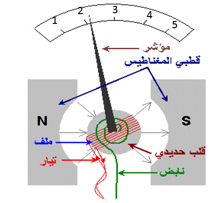
الجلفانوميتر: جهاز يقيس شدة التيار الكهربائي وفرق الجهد.
The galvanometer: an instrument that measures current and potential difference.
الجلفانوميتر في الشكل يقيس شدة التيار. ما قراءة المؤشر؟ وكم رقمًا معنويًا فيها؟
The galvanometer in the figure measures current. What is the pointer reading, and how many significant figures does it have?
📚 قواعد تحديد الأرقام المعنوية
📚 Rules for counting significant figures
| القاعدةRule | المثالExample | عدد الأرقام المعنويةCount |
|---|---|---|
| 1. جميع الأرقام غير الصفرية معنوية.1. All non-zero digits are significant. | \(3.46\) | ثلاثة (\(3,4,6\))three (\(3,4,6\)) |
| 2. الأصفار على يسار العدد (قبل أول رقم غير صفري) ليست معنوية.2. Zeros on the left (before the first non-zero digit) are not significant. | \(0.00034\) | اثنان (\(3,4\))two (\(3,4\)) |
| 3. الأصفار على يمين العدد الصحيح (بلا فاصلة عشرية) ليست معنوية.3. Zeros on the right of a whole number (with no decimal point) are not significant. | \(5800\) | اثنان (\(5,8\))two (\(5,8\)) |
| 4. الأصفار بين رقمين غير صفريين معنوية.4. Zeros between non-zero digits are significant. | \(5003\) | أربعة (\(5,0,0,3\))four (\(5,0,0,3\)) |
| 5. الأصفار بعد الفاصلة العشرية (في نهاية العدد) معنوية.5. Zeros after the decimal point (at the end of the number) are significant. | \(6.00\) | ثلاثة (\(6,0,0\))three (\(6,0,0\)) |
🧠 توضيح إضافي: لماذا هذه القواعد؟
🧠 Extra explanation: why these rules?
الأصفار التي على اليسار (\(0.00034\)) تُحدّد فقط موضع الفاصلة؛ لو غيّرنا الوحدة إلى \(0.34\ mm\) لاختفت ولم تتغيّر دقة القياس. أما الأصفار في النهاية بعد الفاصلة (\(6.00\)) فنكتبها عمدًا لأن القائس قرأها فعلًا: \(6.00\) تعني أن الجهاز دقيق إلى جزء من مئة.
The zeros on the left (\(0.00034\)) only locate the decimal point\; changing the unit to \(0.34\ mm\) removes them without changing the precision of the measurement. Trailing zeros after the point (\(6.00\)) are written on purpose because the person measuring actually read them: \(6.00\) means the instrument resolves to a hundredth.
أما العدد \(5800\) فغامض: هل الصفران مقيسان أم لمجرد تحديد المنزلة؟ نتفق في هذا المنهج على أنهما ليسا معنويين. ولإزالة الغموض نستعمل الترميز العلمي: \(5.8\times10^{3}\) (رقمان) و\(5.80\times10^{3}\) (ثلاثة) و\(5.800\times10^{3}\) (أربعة).
The number \(5800\) is ambiguous: were the two zeros measured or do they just fix the place value? In this course we agree they are not significant. To remove ambiguity we use scientific notation: \(5.8\times10^{3}\) (two), \(5.80\times10^{3}\) (three) and \(5.800\times10^{3}\) (four).
وفي الترميز العلمي تُعدّ كل أرقام \(a\) معنوية. فالترميز العلمي يحافظ على الأرقام المعنوية كما هي.
In scientific notation all the digits of \(a\) are significant, so scientific notation preserves the significant figures exactly.
اكتب أي عدد في التجربة التالية لترى أي أرقامه معنوية والقاعدة التي تنطبق على كل رقم.
Type any number in the next experiment to see which of its digits are significant and which rule applies to each digit.
🧪 تجربة 5: عدّاد الأرقام المعنوية
🧪 Experiment 5: The significant-figures counter
اكتب عددًا (يمكن أن يحوي فاصلة عشرية أو بصيغة مثل \(5.80e3\))، أو اختر مثالًا. تُلوَّن الأرقام المعنوية بالأخضر وغير المعنوية بالرمادي مع رقم القاعدة المنطبقة على كل رقم.
Type a number (it may contain a decimal point or be written like \(5.80e3\)) or choose an example. Significant digits are coloured green and non-significant ones grey, with the number of the rule that applies to each digit.
✍️ قيّم نفسك: عدد الأرقام المعنوية
✍️ Self-check: counting significant figures
كم رقمًا معنويًا في العدد \(0.00520\)؟
How many significant figures does \(0.00520\) have?
كم رقمًا معنويًا في العدد \(2010\)؟
How many significant figures does \(2010\) have?
كم رقمًا معنويًا في العدد \(2.000\)؟
How many significant figures does \(2.000\) have?
كم رقمًا معنويًا في العدد \(98790\)؟
How many significant figures does \(98790\) have?
🧮 الأرقام المعنوية في العمليات الحسابية
🧮 Significant figures in calculations
لا يجوز أن تكون نتيجة الحساب أدقّ من أقل المعطيات دقة. لذلك نحسب أولًا ثم نقرّب الناتج حسب القاعدة المناسبة.
A calculated result cannot be more precise than the least precise data. So we first calculate, then round the result according to the proper rule.
⚖️ قاعدتا العمليات
⚖️ The two rules for operations
الضرب والقسمة: يحتوي الناتج على أرقام معنوية تساوي أقل عدد أرقام معنوية بين المعطيات.
Multiplication and division: the result has as many significant figures as the data value with the fewest significant figures.
مثال: \(\dfrac{1.0}{14.366}=0.0696\;\to\;0.070\) (رقمان معنويان لأن \(1.0\) فيه رقمان).
Example: \(\dfrac{1.0}{14.366}=0.0696\;\to\;0.070\) (two significant figures because \(1.0\) has two).
الجمع والطرح: نقرّب الناتج إلى أقل عدد من المنازل العشرية (الأرقام بعد الفاصلة) بين المعطيات.
Addition and subtraction: round the result to the fewest decimal places (digits after the point) among the data.
مثال: \(1.367+13.2=14.567\;\to\;14.6\) (منزلة عشرية واحدة لأن \(13.2\) فيه منزلة واحدة). والطرح بالقاعدة نفسها.
Example: \(1.367+13.2=14.567\;\to\;14.6\) (one decimal place because \(13.2\) has one). Subtraction follows the same rule.
✂️ قاعدة التقريب
✂️ The rounding rule
ننظر إلى أول رقم سيُحذف: إن كان من \(0\) إلى \(4\) نحذفه ونحذف ما بعده ويبقى الرقم السابق كما هو، وإن كان من \(5\) إلى \(9\) نحذفه ونضيف \(1\) إلى الرقم الذي قبله. مثال: \(2.3456\) إلى ثلاثة أرقام معنوية \(\to\ 2.35\) (الرقم المحذوف \(5\)).
Look at the first digit to be dropped: if it is from \(0\) to \(4\) drop it (and what follows) and leave the previous digit unchanged\; if it is from \(5\) to \(9\) drop it and add \(1\) to the previous digit. Example: \(2.3456\) to three significant figures \(\to\ 2.35\) (the dropped digit is \(5\)).
جرّب العمليات الأربع في التجربة التالية ولاحظ أي قاعدة تُطبَّق وكيف يُقرَّب الناتج.
Try the four operations in the next experiment and notice which rule applies and how the result is rounded.
🧪 تجربة 6: الأرقام المعنوية في العمليات الحسابية
🧪 Experiment 6: Significant figures in calculations
أدخل عددين واختر العملية. يعرض البرنامج الناتج الدقيق على الآلة الحاسبة ثم القاعدة المنطبقة (أقل أرقام معنوية أو أقل منازل عشرية) ثم الناتج بعد التقريب.
Enter two numbers and choose the operation. The program shows the exact calculator result, the rule that applies (fewest significant figures or fewest decimal places) and the rounded result.
باستخدام قواعد الأرقام المعنوية والترميز العلمي، ناتج الضرب \(50.4\times310\) هو:
Using the rules of significant figures and scientific notation, the product \(50.4\times310\) is:
باستخدام قواعد الأرقام المعنوية، ناتج \(5.63+15.1+14\) هو:
Using the rules of significant figures, \(5.63+15.1+14\) equals:
🎯 الدقة والضبط
🎯 Accuracy and Precision
📘 التعريفان
📘 The two definitions
الدقة (Accuracy): مدى قرب القيمة المقاسة من القيمة الحقيقية؛ كلما اقتربت منها كان القياس دقيقًا.
Accuracy: how close the measured value is to the true value; the closer, the more accurate the measurement.
الضبط (Precision): مدى قرب القيم المقاسة من بعضها البعض عند تكرار القياس، بغض النظر عن قربها من القيمة الحقيقية.
Precision: how close the measured values are to one another when the measurement is repeated, whatever their closeness to the true value.
الزمن اللازم لسقوط جسم من ارتفاع \(2\ m\) يساوي \(t=\sqrt{\dfrac{2h}{g}}=\sqrt{\dfrac{2\times2}{9.8}}\approx0.64\ s\). قاس ثلاثة طلاب هذا الزمن وكرّر كلٌّ منهم القياس ثلاث مرات:
The time for an object to fall from a height of \(2\ m\) is \(t=\sqrt{\dfrac{2h}{g}}=\sqrt{\dfrac{2\times2}{9.8}}\approx0.64\ s\). Three students measured this time, each repeating the measurement three times:
| الطالبStudent | القياسات (s)Measurements (s) | المتوسط (s)Mean (s) | أكبر فرق بين قياسين (s)Largest spread (s) | الحكمVerdict |
|---|---|---|---|---|
| أحمدAhmed | \(0.68,\ 0.51,\ 0.95\) | \(0.71\) | \(0.44\) | غير دقيق وغير مضبوطneither accurate nor precise |
| ماجدMajed | \(0.77,\ 0.75,\ 0.76\) | \(0.76\) | \(0.02\) | غير دقيق ولكن مضبوطnot accurate but precise |
| يوسفYousef | \(0.65,\ 0.64,\ 0.63\) | \(0.64\) | \(0.02\) | دقيق ومضبوطaccurate and precise |
🧠 توضيح: تشبيه الهدف
🧠 Clarification: the target analogy
تخيّل رمي سهام نحو لوحة: مركز اللوحة هو القيمة الحقيقية. إن تجمّعت السهام معًا (ضبط عالٍ) لكنها بعيدة عن المركز فالقياس مضبوط غير دقيق، وهذا يدل غالبًا على خطأ منتظم (جهاز غير معايَر مثلًا). وإن انتشرت السهام حول المركز فالقياس دقيق في المتوسط لكنه غير مضبوط، وهذا يدل على خطأ عشوائي. وتكرار القياس وأخذ المتوسط يقلّل الخطأ العشوائي لكنه لا يعالج الخطأ المنتظم.
Imagine throwing darts at a board: the bullseye is the true value. If the darts cluster together (high precision) but away from the centre, the measurement is precise but not accurate, which usually points to a systematic error (an uncalibrated instrument, say). If the darts scatter around the centre the measurement is accurate on average but not precise, pointing to random error. Repeating and averaging reduces the random error but does not cure the systematic one.
غيّر الخطأ المنتظم والتشتت في التجربة التالية لترى الحالات الأربع.
Change the systematic error and the scatter in the next experiment to see all four cases.
🧪 تجربة 7: الدقة والضبط: لوحة الهدف
🧪 Experiment 7: Accuracy and precision: the target board
مركز اللوحة هو القيمة الحقيقية. غيّر الخطأ المنتظم (إزاحة جميع القياسات في اتجاه واحد) والتشتت العشوائي، وراقب كيف تتغيّر الحالة بين دقيق ومضبوط. اضغط «رمي جديد» لتوليد قياسات جديدة بالإعدادات نفسها.
The centre of the board is the true value. Change the systematic error (shifting all the measurements in one direction) and the random scatter, and watch the case change between accurate and precise. Press “New throw” to generate new measurements with the same settings.
قيمة حقيقية لكمية تساوي \(10.0\ cm\). قاس طالب أربع مرات فحصل على \(12.1,\ 12.0,\ 12.2,\ 12.1\ cm\). قياسات الطالب:
The true value of a quantity is \(10.0\ cm\). A student measured four times and got \(12.1,\ 12.0,\ 12.2,\ 12.1\ cm\). The student’s measurements are:
📏 القياس وهامش الخطأ
📏 Measurement and Margin of Error
نقرأ الأجهزة من خلال التدريجات الواضحة عليها. ولكل قراءة هامش خطأ يساوي أصغر تدريجة في الجهاز ÷ 2، ونكتب القراءة على الصورة القراءة ± هامش الخطأ.
We read instruments through the clear divisions on them. Every reading has a margin of error equal to the smallest division of the instrument ÷ 2, and we write the reading as reading ± margin of error.
📌 هامش الخطأ
📌 The margin of error
\[\Delta x=\pm\dfrac{\delta}{2}\]
حيث \(\delta\) أصغر تدريجة في الجهاز. معنى \(2.7\pm0.5\): القيمة الحقيقية موجودة في المدى من \(2.2\) إلى \(3.2\).
where \(\delta\) is the smallest division of the instrument. The meaning of \(2.7\pm0.5\): the true value lies in the range from \(2.2\) to \(3.2\).
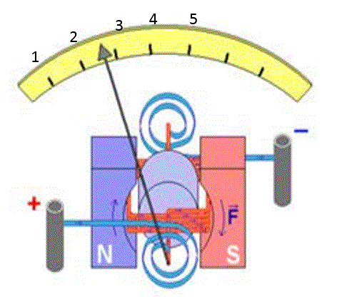
جهاز بتدريج من \(1\) إلى \(5\): المؤشر قرب \(2.7\).
An instrument graduated from \(1\) to \(5\): the pointer is near \(2.7\).
ما قراءة الجهاز في الشكل أعلاه؟ وما هامش الخطأ؟
What is the reading of the instrument in the figure above, and what is the margin of error?
🔗 ربط بمثال القلم
🔗 Link to the pencil example
مسطرة أصغر تدريجة فيها \(1\ mm=0.1\ cm\): هامش الخطأ \(\dfrac{0.1}{2}=0.05\ cm\). لذلك نكتب طول القلم \(13.85\pm0.05\ cm\)، ويظهر هنا لماذا كانت الخانة الأخيرة (\(5\)) هي المقدَّرة: هامش الخطأ في خانة جزء من مئة.
For a ruler whose smallest division is \(1\ mm=0.1\ cm\) the margin is \(\dfrac{0.1}{2}=0.05\ cm\). So we write the pencil length as \(13.85\pm0.05\ cm\), which shows why the last digit (\(5\)) is the estimated one: the margin of error is in the hundredths place.
حرّك الجسم على المسطرة وغيّر أصغر تدريجة لترى كيف يتغيّر هامش الخطأ.
Slide the object along the ruler and change the smallest division to see how the margin of error changes.
🧪 تجربة 8: المسطرة وهامش الخطأ
🧪 Experiment 8: The ruler and the margin of error
حرّك طرف القلم على المسطرة بالمنزلق، واختر أصغر تدريجة في المسطرة. يكتب البرنامج القراءة مع هامش الخطأ (أصغر تدريجة ÷ 2) ويبيّن المدى الممكن للقيمة.
Slide the pencil tip along the ruler with the slider and choose the smallest division of the ruler. The program writes the reading with its margin of error (smallest division ÷ 2) and shows the possible range of the value.
قِيس طول بمسطرة أصغر تدريجة فيها \(0.2\ cm\) فكانت القراءة \(7.4\ cm\). تُكتب القراءة مع هامش الخطأ:
A length is measured with a ruler whose smallest division is \(0.2\ cm\) and the reading is \(7.4\ cm\). The reading with its margin of error is written:
📊 تمثيل البيانات بيانيًا
📊 Representing Data Graphically
❓ ما الغاية من الخط البياني؟
❓ What is the purpose of a graph?
- إظهار العلاقة بين كميتين بنظرة واحدة (طردية؟ عكسية؟ خطية؟).Showing the relation between two quantities at a glance (direct? inverse? linear?).
- التنبؤ بقيم لم نقسها: بين قيمنا (استكمال داخلي) أو بعدها (استكمال خارجي).Predicting values we did not measure: between our values (interpolation) or beyond them (extrapolation).
- استخراج كميات فيزيائية من الميل ومن نقطة تقاطع الخط مع المحور الرأسي.Extracting physical quantities from the slope and from the intercept with the vertical axis.
أي المتغيرات على أي محور؟ نضع على المحور الأفقي القيم التي تحكّمنا بها وتسمّى المتغير المستقل، ونضع على المحور الرأسي القيم التي تغيّرت نتيجة ذلك وتسمّى المتغير التابع.
Which variable on which axis? On the horizontal axis we put the values we controlled, called the independent variable; on the vertical axis we put the values that changed as a result, called the dependent variable.
🕰️ تجربة البندول
🕰️ The pendulum experiment
اضبط البندول على طول معيّن وقِس زمن عشر اهتزازات ثم اقسمه على \(10\) لتحصل على الزمن الدوري \(T\) (قسمة الزمن على عدد كبير من الاهتزازات تقلّل خطأ القياس). كرّر ذلك لأطوال مختلفة. الطول \(L\) هو المتغير المستقل (أفقي) والزمن الدوري \(T\) هو التابع (رأسي).
Set the pendulum to a certain length and measure the time of ten oscillations, then divide by \(10\) to get the period \(T\) (dividing the time of many oscillations reduces the measurement error). Repeat for different lengths. The length \(L\) is the independent variable (horizontal) and the period \(T\) is the dependent one (vertical).
🧪 تجربة 9: تجربة البندول: جدول وخط بياني
🧪 Experiment 9: The pendulum: table and graph
اضبط طول البندول واضغط «قس 10 اهتزازات»؛ يسجّل البرنامج الطول وزمن عشر اهتزازات (مع خطأ قياس صغير عشوائي) ويحسب الزمن الدوري، ثم يضيف نقطة إلى الخط البياني. أضف عدة نقاط (أو اضغط «أضف 6 قياسات») وبدّل بين رسم \(T\) و\(T^{2}\) مقابل \(L\). يحسب البرنامج ميل الخط المستقيم لـ \(T^{2}\) وقيمة \(g\) منه، ويتيح لك التنبؤ بالزمن الدوري لأي طول.
Set the pendulum length and press “Time 10 oscillations”; the program records the length and the time of ten oscillations (with a small random measurement error), computes the period and adds a point to the graph. Add several points (or press “Add 6 trials”) and switch between plotting \(T\) and \(T^{2}\) versus \(L\). The program finds the slope of the \(T^{2}\) line and the value of \(g\) from it, and lets you predict the period for any length.
(1) هل يمكن تحديد الزمن الدوري بدقة لطول بندول غير موجود في الجدول؟ (2) وهل يمكن ذلك من الخط البياني؟ (3) وهل يمكن توقّع الزمن الدوري لطول بندول كبير غير موجود في الجدول؟
(1) Can the period be determined exactly for a pendulum length not in the table? (2) Can it be from the graph? (3) Can we predict the period of a very long pendulum that is not in the table?
🧠 توضيح إضافي: تحويل المنحنى إلى خط مستقيم
🧠 Extra explanation: turning a curve into a straight line
الرسم \(T\) مقابل \(L\) منحنٍ لأن \(T=2\pi\sqrt{L/g}\). وبتربيع الطرفين: \(T^{2}=\dfrac{4\pi^{2}}{g}\,L\)، فإذا رسمنا \(T^{2}\) مقابل \(L\) حصلنا على خط مستقيم يمرّ بنقطة الأصل ميله \(\dfrac{4\pi^{2}}{g}\approx4.0\ s^{2}/m\). ومن الميل نحسب العجلة الأرضية: \(g=\dfrac{4\pi^{2}}{k}\) حيث \(k\) ميل الخط. بدّل بين الرسمين في التجربة أعلاه.
The plot of \(T\) versus \(L\) is a curve because \(T=2\pi\sqrt{L/g}\). Squaring both sides: \(T^{2}=\dfrac{4\pi^{2}}{g}\,L\), so plotting \(T^{2}\) versus \(L\) gives a straight line through the origin with slope \(\dfrac{4\pi^{2}}{g}\approx4.0\ s^{2}/m\). From the slope we find the gravitational acceleration: \(g=\dfrac{4\pi^{2}}{k}\) where \(k\) is the slope of the line. Switch between the two plots in the experiment above.
⚖️ الميل: الكتلة والحجم
⚖️ The slope: mass and volume
درسنا العلاقة بين الحجم والكتلة لمجموعة كتل من النوع نفسه فحصلنا على القيم الآتية، وارسم الخط بوضع الكتلة (المتغير المستقل) على المحور الأفقي والحجم على الرأسي:
We studied the relation between volume and mass for a set of masses of the same material and obtained the values below; plot them with the mass (the independent variable) on the horizontal axis and the volume on the vertical one:
| رقم التجربةTrial | الكتلة \(m\) (kg)Mass \(m\) (kg) | الحجم \(V\) (m³)Volume \(V\) (m³) |
|---|---|---|
| 1 | 1 | 2 |
| 2 | 2 | 4 |
| 3 | 3 | 6 |
| 4 | 4 | 8 |
| 5 | 5 | 10 |
| 6 | 6 | 12 |
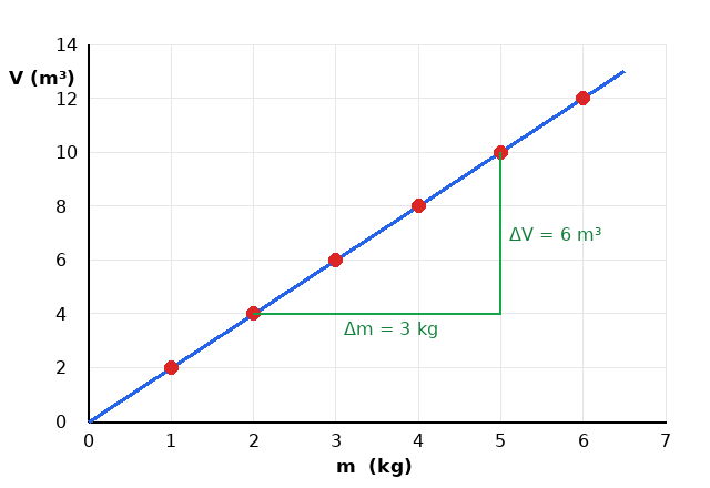
الحجم مقابل الكتلة: خط مستقيم يمرّ بنقطة الأصل.
Volume versus mass: a straight line through the origin.
من الخط البياني احسب ميل الخط، ثم احسب كثافة المادة.
From the graph find the slope of the line, then the density of the material.
🚗 العلاقة الطردية والعلاقة الخطية
🚗 Direct and linear relations
تتحرك سيارة بسرعة ثابتة. إذا بدأت من نقطة الأصل ورسمنا العلاقة بين موقعها والزمن حصلنا على خط مستقيم يمرّ بنقطة الأصل، فنقول إن العلاقة بين الموقع والزمن طردية. وإن بدأت السيارة بعيدًا عن نقطة الأصل فالخط مستقيم لكنه لا يمرّ بنقطة الأصل فنقول إن العلاقة خطية.
A car moves at constant speed. If it starts from the origin and we plot its position against time we get a straight line through the origin, so the relation between position and time is direct. If the car starts away from the origin, the line is straight but does not pass through the origin, and the relation is linear.
📐 معادلات الخط المستقيم
📐 Equations of the straight line
العلاقة الطردية:
Direct relation:
\[y=m\,x\]
العلاقة الخطية:
Linear relation:
\[y=m\,x+b\]
\[m=\dfrac{y_{2}-y_{1}}{x_{2}-x_{1}}\]
وفي منحنى الموقع–الزمن يكون الميل \(m=\dfrac{x_{2}-x_{1}}{t_{2}-t_{1}}=v\) أي السرعة.
For a position–time graph the slope \(m=\dfrac{x_{2}-x_{1}}{t_{2}-t_{1}}=v\) is the speed.
\(m\) هو ميل الخط، و\(b\) هي نقطة تقاطع الخط مع المحور الرأسي (الموقع الابتدائي). العلاقة الطردية حالة خاصة من الخطية حين \(b=0\).
\(m\) is the slope of the line and \(b\) is its intercept with the vertical axis (the initial position). A direct relation is the special case of a linear one with \(b=0\).
غيّر الموقع الابتدائي والسرعة في التجربة التالية وراقب الخط ومعادلته (وهي تحلّ محل محاكاة GeoGebra «رسم الخط البياني ومعادلة الخط»).
Change the initial position and the speed in the next experiment and watch the line and its equation (it replaces the GeoGebra simulation “drawing the graph and its equation”).
🧪 تجربة 10: سيارة بسرعة ثابتة: الموقع والزمن
🧪 Experiment 10: A car at constant speed: position and time
غيّر الموقع الابتدائي \(x_{0}\) والسرعة \(v\) ثم شغّل الحركة. يُرسم الخط البياني للموقع مقابل الزمن ويكتب البرنامج معادلته: الميل هو السرعة، ونقطة تقاطعه مع المحور الرأسي هي الموقع الابتدائي. ويحدّد البرنامج هل العلاقة طردية أم خطية.
Change the initial position \(x_{0}\) and the speed \(v\) then run the motion. The position–time graph is drawn and the program writes its equation: the slope is the speed and the intercept with the vertical axis is the initial position. The program tells whether the relation is direct or linear.
🔁 العلاقة العكسية
🔁 The inverse relation
قد يكون الخط البياني منحنيًا كما في الشكل، وقد تكون العلاقة عكسية. للتأكد نطبّق العلاقة \(\dfrac{y_{1}}{y_{2}}=\dfrac{x_{2}}{x_{1}}\) (أي أن حاصل الضرب \(x\,y\) ثابت)، فإذا تحققت قلنا العلاقة عكسية.
The graph may be a curve, as in the figure, and the relation may be inverse. To check, we apply \(\dfrac{y_{1}}{y_{2}}=\dfrac{x_{2}}{x_{1}}\) (that is, the product \(x\,y\) is constant); if it holds the relation is inverse.
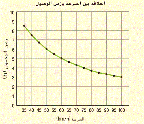
العلاقة بين السرعة (km/h) وزمن الوصول (h): منحنى متناقص.
The relation between speed (km/h) and arrival time (h): a decreasing curve.
هل العلاقة بين السرعة وزمن الوصول في الشكل عكسية؟
Is the relation between speed and arrival time in the figure inverse?
🧪 تجربة 11: العلاقة العكسية: السرعة وزمن الوصول
🧪 Experiment 11: The inverse relation: speed and arrival time
تسافر سيارة مسافة ثابتة \(300\ km\). غيّر السرعة وانظر الزمن \(t=\dfrac{300}{v}\): كلما زادت السرعة نقص الزمن، وحاصل ضربهما ثابت دائمًا. اضغط «سجّل نقطة» لتسجيل نقطتين ومقارنة النسبتين \(\dfrac{y_{1}}{y_{2}}\) و\(\dfrac{x_{2}}{x_{1}}\).
A car travels a fixed distance of \(300\ km\). Change the speed and watch the time \(t=\dfrac{300}{v}\): the higher the speed the shorter the time, and their product is always constant. Press “Record a point” to record two points and compare the ratios \(\dfrac{y_{1}}{y_{2}}\) and \(\dfrac{x_{2}}{x_{1}}\).
| نوع العلاقةRelation | شكل الخطGraph | الصيغةFormula | اختبار سريعQuick test |
|---|---|---|---|
| طرديةDirect | مستقيم يمرّ بنقطة الأصلstraight line through the origin | \(y=m\,x\) | \(y/x\) ثابت\(y/x\) is constant |
| خطيةLinear | مستقيم لا يمرّ بنقطة الأصلstraight line, not through the origin | \(y=m\,x+b\) | الميل ثابتthe slope is constant |
| عكسيةInverse | منحنى متناقص (قطع زائد)a decreasing curve (hyperbola) | \(y=\dfrac{k}{x}\) | \(x\,y\) ثابت\(x\,y\) is constant |
في الجدول التالي: \((x,y)=(2,12),\ (4,6),\ (6,4)\). العلاقة بين \(x\) و\(y\):
In the table \((x,y)=(2,12),\ (4,6),\ (6,4)\). The relation between \(x\) and \(y\) is:
خط بياني للموقع \(x\) مقابل الزمن \(t\) يمرّ بالنقطتين \((t,x)=(1\ s,\ 7\ m)\) و\((5\ s,\ 19\ m)\). سرعة الجسم (ميل الخط) تساوي:
A position \(x\) versus time \(t\) graph passes through the points \((t,x)=(1\ s,\ 7\ m)\) and \((5\ s,\ 19\ m)\). The speed of the object (the slope) is:
📝 ملخص الدرس
📝 Lesson Summary
أهم ما تعلّمناه
Key points
- الترميز العلمي: \(a\times10^{n}\) مع \(1\le a\lt 10\)؛ الأس موجب للأعداد الكبيرة وسالب للصغيرة.Scientific notation: \(a\times10^{n}\) with \(1\le a\lt 10\); the exponent is positive for large numbers and negative for small ones.
- سبع كميات أساسية في النظام الدولي: \(m,\ kg,\ s,\ K,\ A,\ cd,\ mol\).Seven base quantities in SI: \(m,\ kg,\ s,\ K,\ A,\ cd,\ mol\).
- البادئات تعني قوى العشرة (\(k=10^{3},\ m=10^{-3},\ \mu=10^{-6},\ n=10^{-9}\)) ونحوّل بمعامل التحويل الذي يساوي \(1\).Prefixes stand for powers of ten (\(k=10^{3},\ m=10^{-3},\ \mu=10^{-6},\ n=10^{-9}\)) and we convert with a conversion factor equal to \(1\).
- التحليل البعدي: وحدة الطرفين متساوية في العلاقة الصحيحة.Dimensional analysis: both sides of a correct relation have the same unit.
- الأرقام المعنوية: غير الصفرية معنوية، وأصفار اليسار لا، وأصفار الوسط نعم، وأصفار اليمين تُحسب فقط إذا كانت بعد الفاصلة. الضرب والقسمة بأقل عدد أرقام معنوية، والجمع والطرح بأقل عدد منازل عشرية.Significant figures: non-zero digits count, left zeros do not, middle zeros do, right zeros count only after the decimal point. Multiply and divide by the fewest significant figures; add and subtract by the fewest decimal places.
- الدقة قرب من القيمة الحقيقية، والضبط قرب القياسات من بعضها؛ وهامش الخطأ = أصغر تدريجة ÷ 2.Accuracy is closeness to the true value, precision is closeness of the measurements to one another; the margin of error = smallest division ÷ 2.
- الخط البياني: مستقل أفقيًا وتابع رأسيًا؛ الطردية \(y=mx\)، والخطية \(y=mx+b\)، والعكسية \(xy=\)ثابت؛ والميل \(=\dfrac{\Delta y}{\Delta x}\).Graphs: independent on the horizontal axis, dependent on the vertical; direct \(y=mx\), linear \(y=mx+b\), inverse \(xy=\)constant; slope \(=\dfrac{\Delta y}{\Delta x}\).
🧪 اختبر نفسك: امتحان من 20 سؤالاً
🧪 Test Yourself: a 20-Question Exam
أنهِ الدرس بالاختبار التفاعلي التالي؛ أسئلته تجمع بين الفهم والحساب وتغطي جميع أقسام الدرس.
Finish with the interactive exam below; its questions mix understanding with calculation and cover every section of the lesson.
اختبار المدخل إلى علم الفيزياء Introduction to Physics Quiz
20 سؤالاً - الترميز العلمي، الوحدات والبادئات، الأرقام المعنوية، الدقة والضبط، والخطوط البيانية 20 Questions - Scientific Notation, Units and Prefixes, Significant Figures, Accuracy and Precision, and Graphs
• عدد الأسئلة: 20 سؤالاً
• مدة الاختبار: 30 دقيقة
• لا يمكنك تغيير إجاباتك أو إعادة الاختبار إلا بعد 24 ساعة من التسليم.
• تأكد من إجاباتك قبل التسليم! 📌 Important Instructions:
• Number of questions: 20 questions
• Quiz duration: 30 minutes
• You cannot change your answers or retake the quiz for 24 hours after submission.
• Make sure of your answers before submitting!
🔗 محاكيات GeoGebra للاستعانة بها عند اللزوم
🔗 GeoGebra Simulations to Use When Needed
اضغط «تشغيل» لتعمل المحاكاة هنا داخل الدرس؛ ويمكن للطالب الرجوع إليها لتجربة الفكرة بطريقة أخرى.
Press “Run” to run the simulation right here inside the lesson; the student can use it to try the idea in another way.